![]()
A collection of functions for sampling and simulating 3D surfaces and objects and estimating metrics like rugosity, fractal dimension, convexity, sphericity, circularity, second moments of area and volume, and more.
The best way to install habtools is through cran.
install.packages("habtools")You can also install the development version from GitHub with:
# install.packages("devtools")
devtools::install_github("jmadinlab/habtools")There are vignettes demonstrating the use of habtools
for digital elevation models (DEMs) and 3D meshes, as well as a vignette
covering fractal dimension methods.
There are currently two data sets accompanying this package.
horseshoe is a DEM of a coral reef in RasterLayer format,
and mcap is a 3D mesh of a coral growing on a reef in
mesh3d format.
The following example calculates height range, rugosity and fractal
dimension of a 2 x 2 m plot of horseshoe.
library(habtools)
library(raster)

# Let's take a subset DEM of size = 2
dem <- dem_crop(horseshoe, x0 = -465, y0 = 1265, L = 2, plot = TRUE)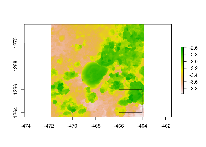
# height range
hr(dem)
#> [1] 1.368289

# rugosity
rg(dem, L0 = 0.0625)
#> [1] 1.75829

# fractal dimension
fd(dem, method = "hvar", keep_data = TRUE, plot=TRUE, diagnose = TRUE)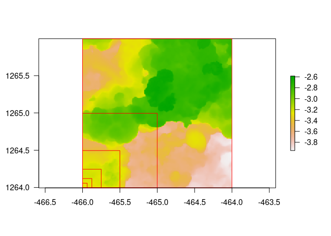
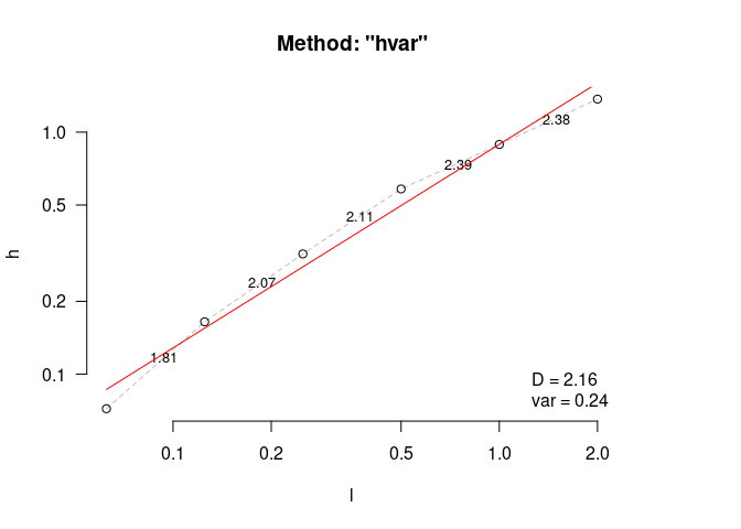
#> $D
#> [1] 2.159332
#>
#> $data
#>        l          h
#> 1 0.0625 0.07207143
#> 2 0.1250 0.16465515
#> 3 0.2500 0.31394699
#> 4 0.5000 0.58224221
#> 5 1.0000 0.88901201
#> 6 2.0000 1.36828852
#>
#> $lvec
#> [1] 0.0625 0.1250 0.2500 0.5000 1.0000 2.0000
#>
#> $D_vec
#> [1] 1.808052 2.068927 2.108902 2.389417 2.377902
#>
#> $var
#> [1] 0.2420993
#>
#> $method
#> [1] "hvar"
The next example calculates height range, rugosity and fractal
dimension for the coral colony mcap. Because 3D meshes can
have more than one z coordinate for a given xy
(i.e., they have overhangs), we use cube counting for fractal
dimension.
library(rgl)
options(rgl.printRglwidget = TRUE)
plot3d(mcap)
# height range
hr(mcap)
#> [1] 0.2185397

# rugosity
rg(mcap, L0 = 0.045)
#> [1] 2.882813

# fractal dimension
fd(mcap, method = "cubes", keep_data = TRUE, plot=TRUE, diagnose = TRUE)
#> lvec is set to c(0.053, 0.106, 0.212, 0.423).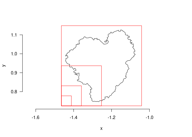
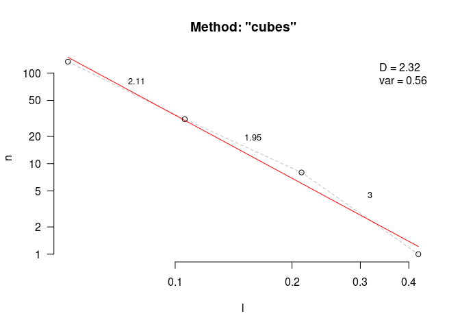
#> $D
#> [1] 2.315246
#>
#> $data
#>            l   n
#> 4 0.05291204 134
#> 3 0.10582408  31
#> 2 0.21164817   8
#> 1 0.42329634   1
#>
#> $lvec
#> [1] 0.42329634 0.21164817 0.10582408 0.05291204
#>
#> $D_vec
#> [1] 2.111893 1.954196 3.000000
#>
#> $var
#> [1] 0.5638126
#>
#> $method
#> [1] "cubes"