rrtableReproducible Research with a Table of R codes
2018-04-15
require(moonBook)
require(ztable)
require(rrtable)
require(ggplot2)If you are a data scientist or researcher, you will certainly be
interested in reproducible research. R package rrtable
makes it possible to make reports with HTML, LaTex, MS word or MS
Powerpoint formats from a table of R codes.
You can install R package rrtable with the following
command.
if(!require(devtools)){ install.packages("devtools") }
devtools::install_github("cardiomoon/rrtable") You can load the rrtable package with the following R
command.
require(rrtable) Sample data sampleData3 is included in rrtable package. You can see the sampleData3 by following R command.
str(sampleData3) 'data.frame': 15 obs. of 5 variables:
$ type : chr "title" "subtitle" "author" "text" ...
$ title : chr "" "" "" "Introduction" ...
$ text : chr "R package `rrtable`" "Reproducible Research with a Table of R codes" "Keon-Woong Moon" "If you are a data scientist or researcher, you will certainly be interested in reproducible research. R package"| __truncated__ ...
$ code : chr "" "" "" "" ...
$ option: chr "" "" "" "" ...You can make a paragraph with this data
df2flextable2( sampleData3 ,vanilla= FALSE )|
type |
title |
text |
code |
option |
|
title |
|
R
package |
|
|
|
subtitle |
|
Reproducible Research with a Table of R codes |
|
|
|
author |
|
Keon-Woong Moon |
|
|
|
text |
Introduction |
If
you are a data scientist or researcher, you will certainly be interested
in reproducible research. R package |
|
|
|
header2 |
Package Installation |
You
can install R package |
if(!require(devtools)){ install.packages(“devtools”) } devtools::install_github(“cardiomoon/rrtable”) |
echo=TRUE, eval=FALSE |
|
header2 |
Package Loading |
You
can load the |
require(rrtable) |
echo=TRUE |
|
header2 |
Sample Data |
Sample data sampleData3 is included in rrtable package. You can see the sampleData3 by following R command. |
str(sampleData3) |
echo=TRUE, eval=TRUE |
|
Data |
Paragraph |
You can make a paragraph with this data |
sampleData3 |
landscape=TRUE |
|
mytable |
mytable object |
You can add mytable object with the following R code. |
mytable(Dx~.,data=acs) |
|
|
plot |
Plot |
You can insert a plot into your document. |
plot(Sepal.Width~Sepal.Length,data=iris) |
|
|
ggplot |
ggplot |
You can insert a ggplot into a document |
ggplot(iris,aes(x=Sepal.Length,y=Sepal.Width,color=Species))+ geom_point() |
|
|
Rcode |
R code |
You can insert the result of R code. For example, you can insert the result of regression analysis. |
fit=lm(mpg~wt*hp,data=mtcars) summary(fit) |
|
|
2ggplots |
Two ggplots |
You can insert two parallel ggplots with the following code. |
ggplot(iris,aes(Sepal.Length,Sepal.Width))+geom_point() ggplot(iris,aes(Sepal.Length,Sepal.Width,colour=Species))+ geom_point()+guides(colour=FALSE) |
|
|
2plots |
Two plots |
You can insert two parallel plots with the following code. |
hist(rnorm(1000)) plot(1:10) |
|
|
header2 |
HTML Report |
You can get report with HTML format(this file) by following R command. |
data2HTML(sampleData3) |
echo=TRUE, eval=FALSE |
You can add mytable object with the following R code.
mytable2flextable( mytable(Dx~.,data=acs) ,vanilla= FALSE )|
Dx |
NSTEMI |
STEMI |
Unstable.Angina |
p |
|
(N=153) |
(N=304) |
(N=400) |
||
|
age |
64.3 ± 12.3 |
62.1 ± 12.1 |
63.8 ± 11.0 |
0.073 |
|
sex |
|
0.012 |
||
|
- Female |
50 (32.7%) |
84 (27.6%) |
153 (38.2%) |
|
|
- Male |
103 (67.3%) |
220 (72.4%) |
247 (61.8%) |
|
|
cardiogenicShock |
|
< 0.001 |
||
|
- No |
149 (97.4%) |
256 (84.2%) |
400 (100.0%) |
|
|
- Yes |
4 ( 2.6%) |
48 (15.8%) |
0 ( 0.0%) |
|
|
entry |
|
0.001 |
||
|
- Femoral |
58 (37.9%) |
133 (43.8%) |
121 (30.2%) |
|
|
- Radial |
95 (62.1%) |
171 (56.2%) |
279 (69.8%) |
|
|
EF |
55.0 ± 9.3 |
52.4 ± 9.5 |
59.2 ± 8.7 |
< 0.001 |
|
height |
163.3 ± 8.2 |
165.1 ± 8.2 |
161.7 ± 9.7 |
< 0.001 |
|
weight |
64.3 ± 10.2 |
65.7 ± 11.6 |
64.5 ± 11.6 |
0.361 |
|
BMI |
24.1 ± 3.2 |
24.0 ± 3.3 |
24.6 ± 3.4 |
0.064 |
|
obesity |
|
0.186 |
||
|
- No |
106 (69.3%) |
209 (68.8%) |
252 (63.0%) |
|
|
- Yes |
47 (30.7%) |
95 (31.2%) |
148 (37.0%) |
|
|
TC |
193.7 ± 53.6 |
183.2 ± 43.4 |
183.5 ± 48.3 |
0.057 |
|
LDLC |
126.1 ± 44.7 |
116.7 ± 39.5 |
112.9 ± 40.4 |
0.004 |
|
HDLC |
38.9 ± 11.9 |
38.5 ± 11.0 |
37.8 ± 10.9 |
0.501 |
|
TG |
130.1 ± 88.5 |
106.5 ± 72.0 |
137.4 ± 101.6 |
< 0.001 |
|
DM |
|
0.209 |
||
|
- No |
96 (62.7%) |
208 (68.4%) |
249 (62.2%) |
|
|
- Yes |
57 (37.3%) |
96 (31.6%) |
151 (37.8%) |
|
|
HBP |
|
0.002 |
||
|
- No |
62 (40.5%) |
150 (49.3%) |
144 (36.0%) |
|
|
- Yes |
91 (59.5%) |
154 (50.7%) |
256 (64.0%) |
|
|
smoking |
|
< 0.001 |
||
|
- Ex-smoker |
42 (27.5%) |
66 (21.7%) |
96 (24.0%) |
|
|
- Never |
50 (32.7%) |
97 (31.9%) |
185 (46.2%) |
|
|
- Smoker |
61 (39.9%) |
141 (46.4%) |
119 (29.8%) |
|
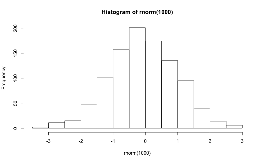
You can insert a plot into your document.
hist(rnorm(1000))
You can insert a ggplot into a document
ggplot(iris,aes(x=Sepal.Length,y=Sepal.Width,color=Species))+ geom_point() 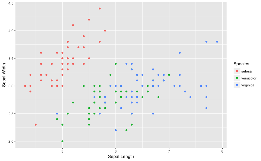
You can insert the result of R code. For example, you can insert the result of regression analysis.
fit=lm(mpg~wt*hp,data=mtcars)
summary(fit)
Call:
lm(formula = mpg ~ wt * hp, data = mtcars)

Residuals:
    Min      1Q  Median      3Q     Max
-3.0632 -1.6491 -0.7362  1.4211  4.5513

Coefficients:
            Estimate Std. Error t value Pr(>|t|)
(Intercept) 49.80842    3.60516  13.816 5.01e-14 ***
wt          -8.21662    1.26971  -6.471 5.20e-07 ***
hp          -0.12010    0.02470  -4.863 4.04e-05 ***
wt:hp        0.02785    0.00742   3.753 0.000811 ***
---
Signif. codes:  0 '***' 0.001 '**' 0.01 '*' 0.05 '.' 0.1 ' ' 1

Residual standard error: 2.153 on 28 degrees of freedom
Multiple R-squared:  0.8848,    Adjusted R-squared:  0.8724
F-statistic: 71.66 on 3 and 28 DF, p-value: 2.981e-13You can insert two parallel ggplots with the following code.
ggplot(iris,aes(Sepal.Length,Sepal.Width))+geom_point()
ggplot(iris,aes(Sepal.Length,Sepal.Width,colour=Species))+ geom_point()+guides(colour=FALSE) 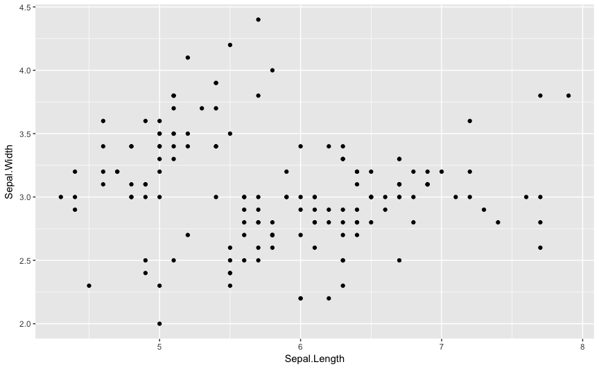
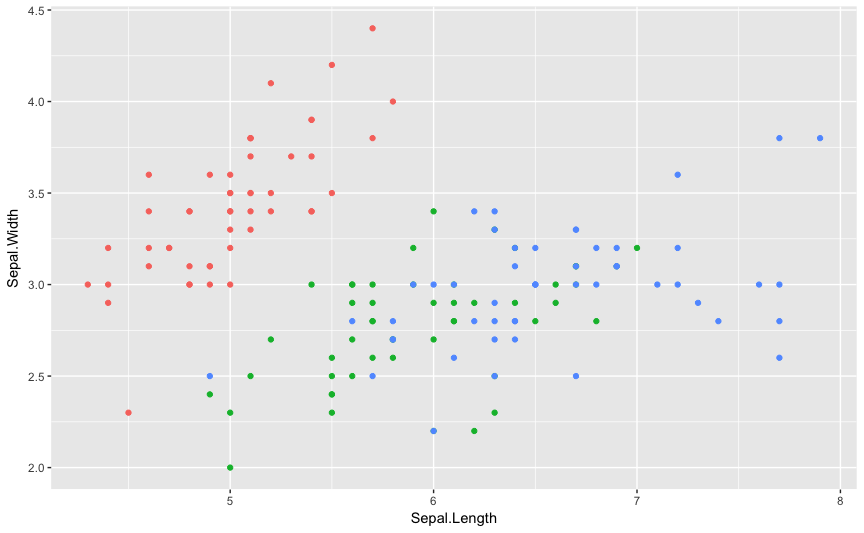
You can insert two parallel plots with the following code.
hist(rnorm(1000))
plot(1:10) 
You can get report with HTML format(this file) by following R command.
data2HTML(sampleData3) You can get a report with MS word format.
data2docx(sampleData3) You can download sample data: sampleData3.docx - view with office web viewer
data2docx(sampleData2) You can download sample data: sampleData2.docx - view with office web viewer
You can get a report with MS word format.
data2pptx(sampleData3) You can download sample data: sampleData3.pptx - view with office web viewer
data2pptx(sampleData2) You can download sample data: sampleData2.pptx - view with office web viewer
You can get a report with pdf format.
data2pdf(sampleData3) You can download sample data: sampleData3.pdf
data2pdf(sampleData2) You can download sample data: sampleData2.pdf